Implementations
In this section we will analyze in detail the basic algorithm techniques used in Machine Learning as well as some applications then used in the various fields of Artificial Intelligence such as Computer Vision, Speech Recognition, Natural Language Processing etc.
K-Nearest Neighbors
How It Works
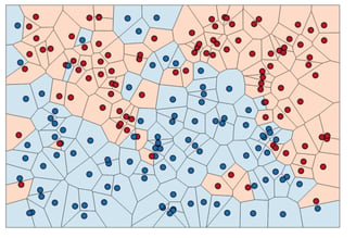
In its simplest version, the k-NN algorithm only considers exactly one nearest neighbor, which is the closest training data point to the point we want to make a prediction for. The prediction is then simply the known output for this training point. Figure below illustrates this for the case of classification on the forge dataset:
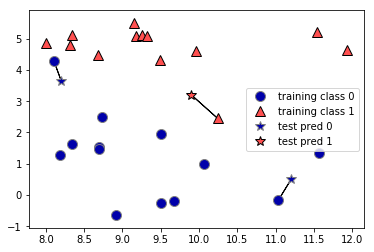
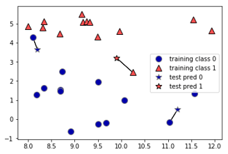
Here, we added three new data points, shown as stars. For each of them, we marked the closest point in the training set. The prediction of the one-nearest-neighbor algorithm is the label of that point (shown by the color of the cross).
Instead of considering only the closest neighbor, we can also consider an arbitrary number, k, of neighbors. This is where the name of the k-nearest neighbors algorithm comes from. When considering more than one neighbor, we use voting to assign a label. This means that for each test point, we count how many neighbors belong to class 0 and how many neighbors belong to class 1. We then assign the class that is more frequent: in other words, the majority class among the k-nearest neighbors. The following example uses the five closest neighbors:
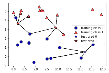
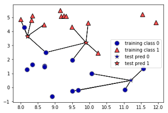
Again, the prediction is shown as the color of the cross. You can see that the prediction for the new data point at the top left is not the same as the prediction when we used only one neighbor.
While this illustration is for a binary classification problem, this method can be applied to datasets with any number of classes. For more classes, we count how many neighbors belong to each class and again predict the most common class.
Implementation From Scratch
Here’s the pseudocode for the kNN algorithm to classify one data point (let’s call it A):
For every point in our dataset:
calculate the distance between A and the current point
sort the distances in increasing order
take k items with lowest distances to A
find the majority class among these items
return the majority class as our prediction for the class of A
The Python code for the function is here:
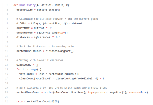
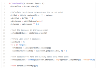
Let’s dig a bit deeper into the code:
The function knnclassify takes 4 inputs: the input vector to classify called A, a full matrix of training examples called dataSet, a vector of labels called labels, and k — the number of nearest neighbors to use in the voting. The labels vector should have as many elements in it as there are rows in the dataSet matrix.
We calculate the distances between A and the current point using the Euclidean distance.
Then we sort the distances in an increasing order.
Next, the lowest k distances are used to vote on the class of A.
After that, we take the classCount dictionary and decompose it into a list of tuples and then sort the tuples by the 2nd item in the tuple. The sort is done in reverse so we have the largest to smallest.
Lastly, we return the label of the item occurring the most frequently.
Implementation Via Scikit-Learn
Now let’s take a look at how we can implement the kNN algorithm using scikit-learn:
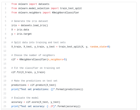
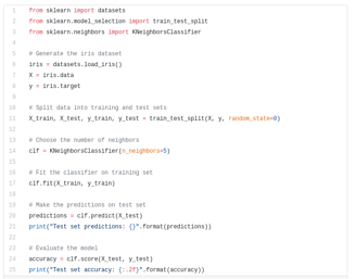
Let’s look into the code:
First, we generate the iris dataset.
Then, we split our data into a training and test set to evaluate generalization performance.
Next, we specify the number of neighbors (k) to 5.
Next, we fit the classifier using the training set.
To make predictions on the test data, we call the predict method. For each data point in the test set, the method computes its nearest neighbors in the training set and finds the most common class among them.
Lastly, we evaluate how well our model generalizes by calling the score method with test data and test labels.
Running the model should gives us a test set accuracy of 97%, meaning the model predicted the class correctly for 97% of the samples in the test dataset.

Strengths and Weaknesses
In principle, there are two important parameters to the KNeighbors classifier: the number of neighbors and how you measure distance between data points.
In practice, using a small number of neighbors like three or five often works well, but you should certainly adjust this parameter.
Choosing the right distance measure is somewhat tricky. By default, Euclidean distance is used, which works well in many settings.
One of the strengths of k-NN is that the model is very easy to understand, and often gives reasonable performance without a lot of adjustments. Using this algorithm is a good baseline method to try before considering more advanced techniques. Building the nearest neighbors model is usually very fast, but when your training set is very large (either in number of features or in number of samples) prediction can be slow. When using the k-NN algorithm, it’s important to preprocess your data. This approach often does not perform well on datasets with many features (hundreds or more), and it does particularly badly with datasets where most features are 0 most of the time (so-called sparse datasets).
In Conclusion
The k-Nearest Neighbors algorithm is a simple and effective way to classify data. It is an example of instance-based learning, where you need to have instances of data close at hand to perform the machine learning algorithm. The algorithm has to carry around the full dataset; for large datasets, this implies a large amount of storage. In addition, you need to calculate the distance measurement for every piece of data in the database, and this can be cumbersome. An additional drawback is that kNN doesn’t give you any idea of the underlying structure of the data; you have no idea what an “average” or “exemplar” instance from each class looks like.
So, while the nearest k-neighbors algorithm is easy to understand, it is not often used in practice, due to prediction being slow and its inability to handle many features.
Reference Sources:
Machine Learning In Action by Peter Harrington (2012)
Introduction to Machine Learning with Python by Sarah Guido and Andreas Muller (2016)
Natural Language Processing
What is NLP?
(NLP) is a field at the intersection of computer science, artificial intelligence, and linguistics. The goal is for computers to process or “understand” natural language in order to perform tasks like Language Translation and Question Answering.
With the rise of voice interfaces and chat-bots, NLP is one of the most important technologies of the information age a crucial part of artificial intelligence. Fully understanding and representing the meaning of language is an extremely difficult goal. Why? Because human language is quite special.
What’s special about human language? A few things actually:
Human language is a system specifically constructed to convey the speaker/writer’s meaning. It’s not just an environmental signal but a deliberate communication. Besides, it uses an encoding that little kids can learn quickly; it also changes.
Human language is mostly a discrete/symbolic/categorical signaling system, presumably because of greater signaling reliability.
The categorical symbols of a language can be encoded as a signal for communication in several ways: sound, gesture, writing, images, etc. human language is capable of being any of those.
Human languages are ambiguous (unlike programming and other formal languages); thus there is a high level of complexity in representing, learning, and using linguistic / situational / contextual / word / visual knowledge towards the human language.
Why study NLP?
There’s a fast-growing collection of useful applications derived from this field of study. They range from simple to complex. Below are a few of them:
Spell Checking, Keyword Search, Finding Synonyms.
Extracting information from websites such as: product price, dates, location, people, or company names.
Classifying: reading level of school texts, positive/negative sentiment of longer documents.
Machine Translation.
Spoken Dialog Systems.
Complex Question Answering.
Indeed, these applications have been used abundantly in industry: from search (written and spoken) to online advertisement matching; from automated/assisted translation to sentiment analysis for marketing or finance/trading; and from speech recognition to chatbots/dialog agents (automating customer support, controlling devices, ordering goods).
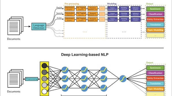

Deep Learning
Most of these NLP technologies are powered by Deep Learning — a subfield of machine learning. Deep Learning only started to gain momentum again at the beginning of this decade, mainly due to these circumstances:
Larger amounts of training data.
Faster machines and multicore CPU/GPUs.
New models and algorithms with advanced capabilities and improved performance: More flexible learning of intermediate representations, more effective end-to-end joint system learning, more effective learning methods for using contexts and transferring between tasks, as well as better regularization and optimization methods.
Most machine learning methods work well because of human-designed representations and input features, along with weight optimization to best make a final prediction. On the other hand, in deep learning, representation learning attempts to automatically learn good features or representations from raw inputs. Manually designed features in machine learning are often over-specified, incomplete, and take a long time to design and validate. In contrast, deep learning’s learned features are easy to adapt and fast to learn.
Deep Learning provides a very flexible, universal, and learnable framework for representing the world, for both visual and linguistic information. Initially, it resulted in breakthroughs in fields such as speech recognition and computer vision. Recently, deep learning approaches have obtained very high performance across many different NLP tasks. These models can often be trained with a single end-to-end model and do not require traditional, task-specific feature engineering.
I recently finished Stanford’s comprehensive CS224n course on Natural Language Processing with Deep Learning. The course provides a thorough introduction to cutting-edge research in deep learning applied to NLP. On the model side, it covers word vector representations, window-based neural networks, recurrent neural networks, long-short-term-memory models, recursive neural networks, and convolutional neural networks, as well as some recent models involving a memory component.
On the programming side, I learned to implement, train, debug, visualize, and invent my own neural network models. In this 2-part series, I want to share the 7 major NLP techniques that I have learned as well as major deep learning models and applications using each of them.
Quick Note: You can access the lectures and programming assignments from CSS 224 at this GitHub Repo.
Technique 1: Text Embeddings
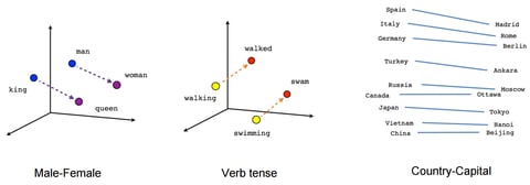
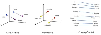
In traditional NLP, we regard words as discrete symbols, which can then be represented by one-hot vectors. A vector’s dimension is the number of words in entire vocabulary. The problem with words as discrete symbols is that there is no natural notion of similarity for one-hot vectors. Thus, the alternative is to learn to encode similarity in the vectors themselves. The core idea is that a word’s meaning is given by the words that frequently appear close by.
Text Embeddings are real valued vector representations of strings. We build a dense vector for each word, chosen so that it’s similar to vectors of words that appear in similar contexts. Word embeddings are considered a great starting point for most deep NLP tasks. They allow deep learning to be effective on smaller datasets, as they are often the first inputs to a deep learning architecture and the most popular way of transfer learning in NLP. The most popular names in word embeddings are Word2vec by Google (Mikolov) and GloVe by Stanford (Pennington, Socher and Manning). Let’s delve deeper into these word representations:
In Word2vec, we have a large corpus of text in which every word in a fixed vocabulary is represented by a vector. We then go through each position t in the text, which has a center word c and context words o. Next, we
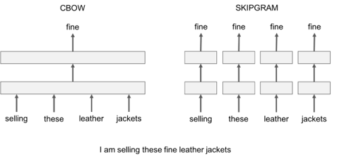
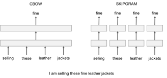
1. Skip-Gram: We consider a context window containing k consecutive terms. Then we skip one of these words and try to learn a neural network that gets all terms except the one skipped and predicts the skipped term. Therefore, if 2 words repeatedly share similar contexts in a large
corpus, the embedding vectors of those terms will have close vectors.
Continuous Bag of Words: We take lots and lots of sentences in a large corpus. Every time we see a word, we take the surrounding word. Then we input the context words to a neural network and predict the word in the center of this context. When we have thousands of such context words and the center word, we have one instance of a dataset for the neural network. We train the neural network and finally the encoded hidden layer output represents the embedding for a particular word. It so happens that when we train this over a large number of sentences, words in similar context get similar vectors.
use the similarity of the word vectors for c and o to calculate the probability of o given c (or vice versa). We keep adjusting the word vectors to maximize this probability.For efficient training of Word2vec, we can eliminate meaningless (or higher frequency) words from the dataset (such as a, the, of, then…). This helps improve model accuracy and training time. Additionally, we can use negative sampling for every input by updating the weights for all the correct labels, but only on a small number of incorrect labels.
Word2vec has 2 model variants worth mentioning:
One grievance with both Skip-Gram and CBOW is such that they are both window-based models, meaning the co-occurrence statistics of the corpus are not used efficiently, resulting in suboptimal embeddings. The GloVe model seeks to solve this problem by capturing the meaning of one word embedding with the structure of the whole observed corpus. To do so, the model One grievance with both Skip-Gram
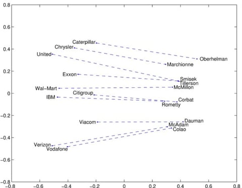
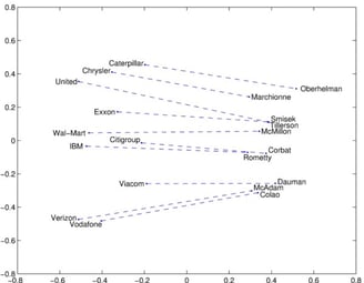
and CBOW is that they’re both window-based models, meaning the co-occurrence statistics of the corpus are not used efficiently, resulting in suboptimal embeddings.The GloVe model seeks to solve this problem by capturing the meaning of one word embedding with the structure of the whole observed corpus. To do so, the model trains on global co-occurrence counts of words and makes a sufficient use of statistics by minimizing least-squares error and, as a result, produces a word vector space with meaningful substructure. Such an outline sufficiently preserves words’ similarities with vector distance.
Besides these 2 text embeddings, there are many more advanced models developed recently, including FastText, Poincare Embeddings, sense2vec, Skip-Thought, Adaptive Skip-Gram. I highly encourage you to check them out.
Technique 2: Machine Translation
Machine Translation is the classic test of language understanding. It consists of both language analysis and language generation. Big machine translation systems have huge commercial use, as global language is a $40 Billion-per-year industry. To give you some notable examples:
Google Translate goes through 100 billion words per day.
Facebook uses machine translation to translate text in posts and comments automatically, in order to break language barriers and allow people around the world to communicate with each other.
eBay uses Machine Translation tech to enable cross-border trade and connect buyers and sellers around the world.
Microsoft brings AI-powered translation to end users and developers on Android, iOS, and Amazon Fire, whether or not they have access to the Internet.
Systran became the 1st software provider to launch a Neural Machine Translation engine in more than 30 languages back in 2016.
In a traditional Machine Translation system, we have to use parallel corpus — a collection of texts, each of which is translated into one or more other languages than the original. For example, given the source language f (e.g. French) and the target language e (e.g. English), we need to build multiple statistical models, including a probabilistic formulation using the Bayesian rule, a translation model p(f|e) trained on the parallel corpus, and a language model p(e) trained on the English-only corpus.
Needless to say, this approach skips hundreds of important details, requires a lot of human feature engineering, consists of many different & independent machine learning problems, and overall is a very complex system.
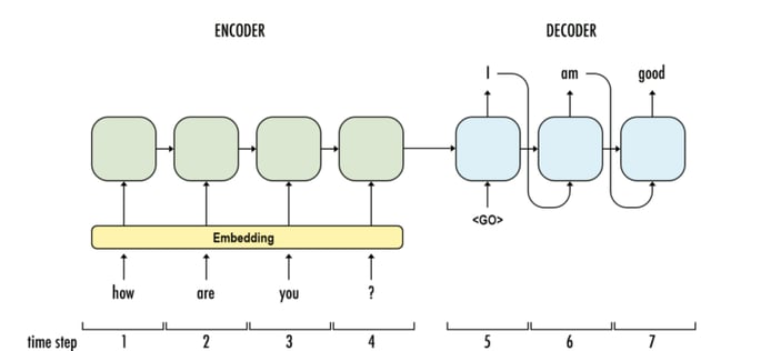
Neural Machine Translation is the approach of modeling this entire process via one big artificial neural network, known as a Recurrent Neural Network(RNN).
RNN is a stateful neural network, in which it has connections between passes, connections through time. Neurons are fed information not just from the previous layer but also from themselves from the previous pass. This means that the order in which we feed the input and train the network matters: feeding it “Donald” and then “Trump” may yield different results compared to feeding it “Trump” and then “Donald”.
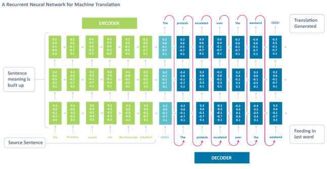
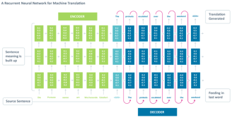
Standard Neural Machine Translation is an end-to-end neural network where the source sentence is encoded by a RNN called encoder, and the target words are predicted using another RNN known as decoder. The RNN Encoder reads a source sentence one symbol at a time, and then summarizes the entire source sentence in its last hidden state. The RNN Decoder uses back-propagation to learn this summary and returns the translated version. It’s amazing that Neural Machine Translation went from a fringe research activity in 2014 to the widely adopted leading way to do Machine Translation in 2016. So what are the big wins of using Neural Machine Translation?
End-to-end training: All parameters in NMT are simultaneously optimized to minimize a loss function on the network’s output.
Distributed representations share strength: NMT has a better exploitation of word and phrase similarities.
Better exploration of context: NMT can use a much bigger context — both source and partial target text — to translate more accurately.
More fluent text generation: Deep learning text generation is of much higher quality than the parallel corpus way.
One big problem with RNNs is the vanishing (or exploding) gradient problem where, depending on the activation functions used, information rapidly gets lost over time. Intuitively, this wouldn’t be much of a problem because these are just weights and not neuron states, but the weights through time is actually where the information from the past is stored; if the weight reaches a value of 0 or 1,000,000, the previous state won’t be very informative. As a consequence, RNNs will experience difficulty in memorizing previous words very far away in the sequence and are only able to make predictions based on the most recent words.
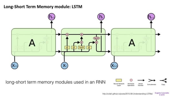
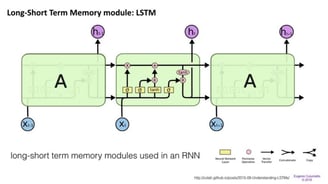
Long / short term memory (LSTM) networks try to combat the vanishing / exploding gradient problem by introducing gates and an explicitly defined memory cell. Each neuron has a memory cell and three gates: input, output and forget. The function of these gates is to safeguard the information by stopping or allowing the flow of it.
The input gate determines how much of the information from the previous layer gets stored in the cell.
The output layer takes the job on the other end and determines how much of the next layer gets to know about the state of this cell.
The forget gate seems like an odd inclusion at first but sometimes it’s good to forget: if it’s learning a book and a new chapter begins, it may be necessary for the network to forget some characters from the previous chapter.
LSTMs have been shown to be able to learn complex sequences, such as writing like Shakespeare or composing primitive music. Note that each of these gates has a weight to a cell in the previous neuron, so they typically require more resources to run. LSTMs are currently very hip and have been used a lot in machine translation. Besides that, It is the default model for most sequence labeling tasks, which have lots and lots of data.
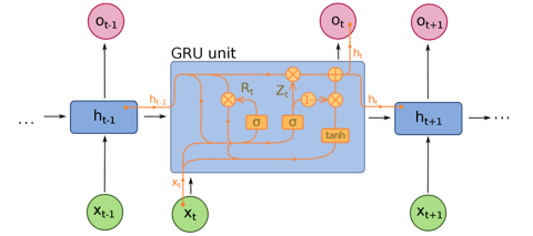
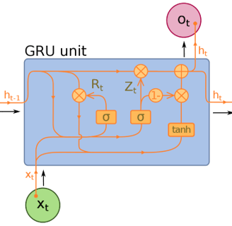
Gated Recurrent Units(GRU) are a slight variation on LSTMs and are also extensions of Neural Machine Translation. They have one less gate and are wired slightly differently: instead of an input, output, and a forget gate, they have an update gate. This update gate determines both how much information to keep from the last state and how much information to let in from the previous layer.
The reset gate functions much like the forget gate of an LSTM, but it’s located slightly differently. They always send out their full state — they don’t have an output gate. In most cases, they function very similarly to LSTMs, with the biggest difference being that GRUs are slightly faster and easier to run (but also slightly less expressive). In practice these tend to cancel each other out, as you need a bigger network to regain some expressiveness, which in turn cancels out the performance benefits. In some cases where the extra expressiveness is not needed, GRUs can outperform LSTMs.
Besides these 3 major architecture, there have been further improvements in neural machine translation system over the past few years. Below are the most notable developments:
Sequence to Sequence Learning with Neural Networks proved the effectiveness of LSTM for Neural Machine Translation. It presents a general end-to-end approach to sequence learning that makes minimal assumptions on the sequence structure. The method uses a multilayered Long Short-Term Memory (LSTM) to map the input sequence to a vector of a fixed dimensionality, and then another deep LSTM to decode the target sequence from the vector.
Neural Machine Translation by Jointly Learning to Align and Translate introduced the attention mechanism in NLP (which will be covered in the next post). Acknowledging that the use of a fixed-length vector is a bottleneck in improving the performance of NMT, the authors propose to extend this by allowing a model to automatically (soft-)search for parts of a source sentence that are relevant to predicting a target word, without having to form these parts as a hard segment explicitly.
Convolutional over Recurrent Encoder for Neural Machine Translation augments the standard RNN encoder in NMT with additional convolutional layers in order to capture wider context in the encoder output.
Google built its own NMT system, called Google’s Neural Machine Translation, which addresses many issues in accuracy and ease of deployment. The model consists of a deep LSTM network with 8 encoder and 8 decoder layers using residual connections as well as attention connections from the decoder network to the encoder.
Instead of using Recurrent Neural Networks, Facebook AI Researchers uses convolutional neural networks for sequence to sequence learning tasks in NMT.
Technique 3: Dialogue and Conversations
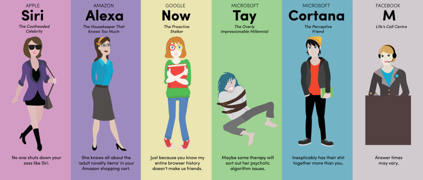
A lot has been written about conversational AI, and a majority of it focuses on vertical chatbots, messenger platforms, business trends, and startup opportunities (think Amazon Alexa, Apple Siri, Facebook M, Google Assistant, Microsoft Cortana). AI’s capability of understanding natural language is still limited. As a result, creating fully-automated, open-domain conversational assistants has remained an open challenge. Nonetheless, the work shown below serve as great starting points for people who want to seek the next breakthrough in conversation AI.

Researchers from Montreal, Georgia Tech, Microsoft and Facebook built a neural network that is capable of generating context-sensitive conversational responses. This novel response generation system can be trained end-to-end on large quantities of unstructured Twitter conversations. A Recurrent Neural Network architecture is used to address sparsity issues that arise when integrating contextual information into classic statistical models, allowing the system to take into account previous dialog utterances. The model shows consistent gains over both context-sensitive and non-context-sensitive Machine Translation and Information Retrieval baselines.
Developed in Hong Kong, Neural Responding Machine (NRM) is a neural-network-based response generator for short-text conversation. It takes the general encoder-decoder framework. First, it formalizes the generation of response as a decoding process based on the latent representation of the input text, while both encoding and decoding are realized with Recurrent Neural Networks. The NRM is trained with a large amount of one-round conversation data collected from a microblogging service. Empirical study shows that NRM can generate grammatically correct and content-wise appropriate responses to over 75% of the input text, outperforming state-of-the-arts in the same setting.

Last but not least, Google’s Neural Conversational Model is a simple approach to conversational modeling. It uses the sequence-to-sequence framework. The model converses by predicting the next sentence given the previous sentence(s) in a conversation. The strength of the model is such it can be trained end-to-end and thus requires much fewer hand-crafted rules.
The model can generate simple conversations given a large conversational training dataset. It is able to extract knowledge from both a domain specific dataset, and from a large, noisy, and general domain dataset of movie subtitles. On a domain-specific IT help-desk dataset, the model can find a solution to a technical problem via conversations. On a noisy open-domain movie transcript dataset, the model can perform simple forms of common sense reasoning.
Semantic Segmentation
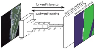
How to Do Semantic Segmentation Using Deep Learning


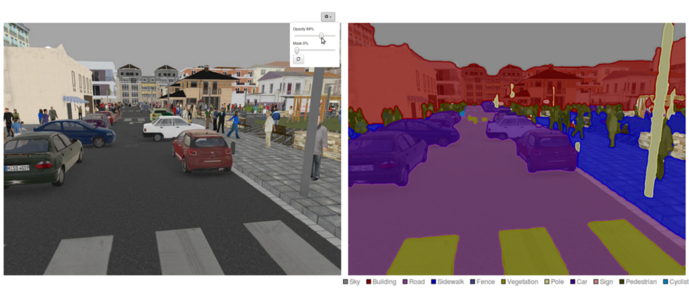
Deeplab Image Semantic Segmentation Network (Source: https://sthalles.github.io/deep_segmentation_network/)
Nowadays, semantic segmentation is one of the key problems in the field of computer vision. Looking at the big picture, semantic segmentation is one of the high-level task that paves the way towards complete scene understanding. The importance of scene understanding as a core computer vision problem is highlighted by the fact that an increasing number of applications nourish from inferring knowledge from imagery. Some of those applications include self-driving vehicles, human-computer interaction, virtual reality etc. With the popularity of deep learning in recent years, many semantic segmentation problems are being tackled using deep architectures, most often Convolutional Neural Nets, which surpass other approaches by a large margin in terms of accuracy and efficiency.
What is Semantic Segmentation?Semantic segmentation is a natural step in the progression from coarse to fine inference:
The origin could be located at classification, which consists of making a prediction for a whole input.
The next step is localization / detection, which provide not only the classes but also additional information regarding the spatial location of those classes.
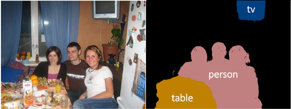
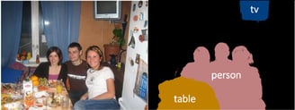
Finally, semantic segmentation achieves fine-grained inference by making dense predictions inferring labels for every pixel, so that each pixel is labeled with the class of its enclosing object ore region.
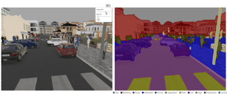
An example of semantic segmentation (Source: https://blog.goodaudience.com/using-convolutional-neural-networks-for-image-segmentation-a-quick-intro-75bd68779225)
It is also worthy to review some standard deep networks that have made significant contributions to the field of computer vision, as they are often used as the basis of semantic segmentation systems:
AlexNet: Toronto’s pioneering deep CNN that won the 2012 ImageNet competition with a test accuracy of 84.6%. It consists of 5 convolutional layers, max-pooling ones, ReLUs as non-linearities, 3 fully-convolutional layers, and dropout.
VGG-16: This Oxford’s model won the 2013 ImageNet competition with 92.7% accuracy. It uses a stack of convolution layers with small receptive fields in the first layers instead of few layers with big receptive fields.
GoogLeNet: This Google’s network won the 2014 ImageNet competition with accuracy of 93.3%. It is composed by 22 layers and a newly introduced building block called inception module. The module consists of a Network-in-Network layer, a pooling operation, a large-sized convolution layer, and small-sized convolution layer.
ResNet: This Microsoft’s model won the 2016 ImageNet competition with 96.4 % accuracy. It is well-known due to its depth (152 layers) and the introduction of residual blocks. The residual blocks address the problem of training a really deep architecture by introducing identity skip connections so that layers can copy their inputs to the next layer.


What are the existing Semantic Segmentation approaches?A general semantic segmentation architecture can be broadly thought of as an encoder network followed by a decoder network:
The encoder is usually is a pre-trained classification network like VGG/ResNet followed by a decoder network.
The task of the decoder is to semantically project the discriminative features (lower resolution) learnt by the encoder onto the pixel space (higher resolution) to get a dense classification.
Unlike classification where the end result of the very deep network is the only important thing, semantic segmentation not only requires discrimination at pixel level but also a mechanism to project the discriminative features learnt at different stages of the encoder onto the pixel space. Different approaches employ different mechanisms as a part of the decoding mechanism. Let’s explore the 3 main approaches:
1 — Region-Based Semantic SegmentationThe region-based methods generally follow the “segmentation using recognition” pipeline, which first extracts free-form regions from an image and describes them, followed by region-based classification. At test time, the region-based predictions are transformed to pixel predictions, usually by labeling a pixel according to the highest scoring region that contains it.
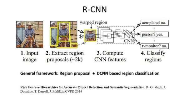

R-CNN (Regions with CNN feature) is one representative work for the region-based methods. It performs the semantic segmentation based on the object detection results. To be specific, R-CNN first utilizes selective search to extract a large quantity of object proposals and then computes CNN features for each of them. Finally, it classifies each region using the class-specific linear SVMs. Compared with traditional CNN structures which are mainly intended for image classification, R-CNN can address more complicated tasks, such as object detection and image segmentation, and it even becomes one important basis for both fields. Moreover, R-CNN can be built on top of any CNN benchmark structures, such as AlexNet, VGG, GoogLeNet, and ResNet.For the image segmentation task, R-CNN extracted 2 types of features for each region: full region feature and foreground feature, and found that it could lead to better performance when concatenating them together as the region feature. R-CNN achieved significant performance improvements due to using the highly discriminative CNN features. However, it also suffers from a couple of drawbacks for the segmentation task:
The feature is not compatible with the segmentation task.
The feature does not contain enough spatial information for precise boundary generation.
Generating segment-based proposals takes time and would greatly affect the final performance.
Due to these bottlenecks, recent research has been proposed to address the problems, including SDS, Hypercolumns, Mask R-CNN.
2 — Fully Convolutional Network-Based Semantic SegmentationThe original Fully Convolutional Network (FCN) learns a mapping from pixels to pixels, without extracting the region proposals. The FCN network pipeline is an extension of the classical CNN. The main idea is to make the classical CNN take as input arbitrary-sized images. The restriction of CNNs to accept and produce labels only for specific sized inputs comes from the fully-connected layers which are fixed. Contrary to them, FCNs only have convolutional and pooling layers which give them the ability to make predictions on arbitrary-sized inputs.
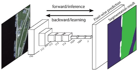
FCN Architecture
For example, Boxsup employed the bounding box annotations as a supervision to train the network and iteratively improve the estimated masks for semantic segmentation. Simple Does It treated the weak supervision limitation as an issue of input label noise and explored recursive training as a de-noising strategy. Pixel-level Labeling interpreted the segmentation task within the multiple-instance learning framework and added an extra layer to constrain the model to assign more weight to important pixels for image-level classification.
Boxsup Training
Doing Semantic Segmentation with Fully-Convolutional Network
In this section, let’s walk through a step-by-step implementation of the most popular architecture for semantic segmentation — the Fully-Convolutional Net (FCN). We’ll implement it using the TensorFlow library in Python 3, along with other dependencies such as Numpy and Scipy.
In this exercise we will label the pixels of a road in images using FCN. We’ll work with the Kitti Road Dataset for road/lane detection. This is a simple exercise from the Udacity’s Self-Driving Car Nano-degree program, which you can learn more about the setup in this GitHub repo.

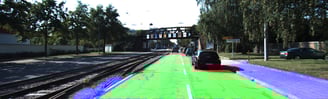
Kitti Road Dataset Training Sample (Source: http://www.cvlibs.net/datasets/kitti/eval_road_detail.php?result=3748e213cf8e0100b7a26198114b3cdc7caa3aff)
Here are the key features of the FCN architecture:
FCN transfers knowledge from VGG16 to perform semantic segmentation.
The fully connected layers of VGG16 is converted to fully convolutional layers, using 1x1 convolution. This process produces a class presence heat map in low resolution.
The upsampling of these low resolution semantic feature maps is done using transposed convolutions (initialized with bilinear interpolation filters).
At each stage, the upsampling process is further refined by adding features from coarser but higher resolution feature maps from lower layers in VGG16.
Skip connection is introduced after each convolution block to enable the subsequent block to extract more abstract, class-salient features from the previously pooled features.
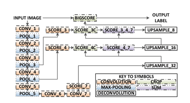
There are 3 versions of FCN (FCN-32, FCN-16, FCN-8). We’ll implement FCN-8, as detailed step-by-step below:
Encoder: A pre-trained VGG16 is used as an encoder. The decoder starts from Layer 7 of VGG16.
FCN Layer-8: The last fully connected layer of VGG16 is replaced by a 1x1 convolution.
FCN Layer-9: FCN Layer-8 is upsampled 2 times to match dimensions with Layer 4 of VGG 16, using transposed convolution with parameters: (kernel=(4,4), stride=(2,2), paddding=’same’). After that, a skip connection was added between Layer 4 of VGG16 and FCN Layer-9.
FCN Layer-10: FCN Layer-9 is upsampled 2 times to match dimensions with Layer 3 of VGG16, using transposed convolution with parameters: (kernel=(4,4), stride=(2,2), paddding=’same’). After that, a skip connection was added between Layer 3 of VGG 16 and FCN Layer-10.
FCN Layer-11: FCN Layer-10 is upsampled 4 times to match dimensions with input image size so we get the actual image back and depth is equal to number of classes, using transposed convolution with parameters: (kernel=(16,16), stride=(8,8), paddding=’same’).
Step 1
We first load the pre-trained VGG-16 model into TensorFlow. Taking in the TensorFlow session and the path to the VGG Folder (which is downloadable here), we return the tuple of tensors from VGG model, including the image input, keep_prob (to control dropout rate), layer 3, layer 4, and layer 7.
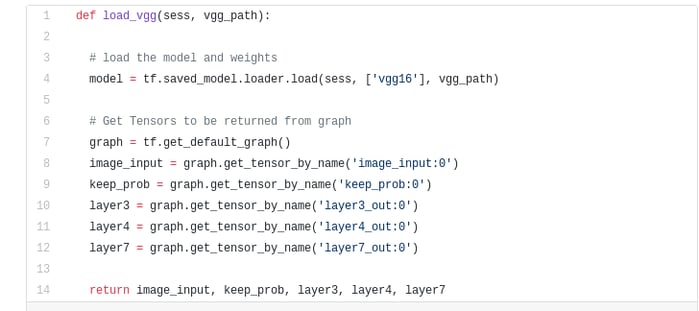
VGG16 Function
Step 2
Now we focus on creating the layers for a FCN, using the tensors from the VGG model. Given the tensors for VGG layer output and the number of classes to classify, we return the tensor for the last layer of that output. In particular, we apply a 1x1 convolution to the encoder layers, and then add decoder layers to the network with skip connections and upsampling.
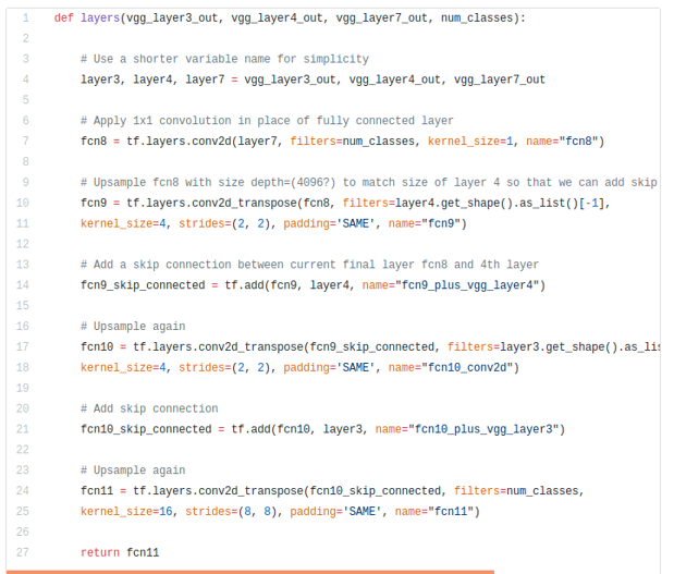
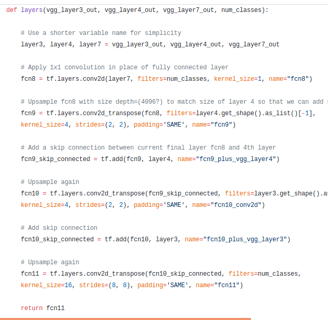
Layers Function
Step 3
The next step is to optimize our neural network, aka building TensorFlow loss functions and optimizer operations. Here we use cross entropy as our loss function and Adam as our optimization algorithm.
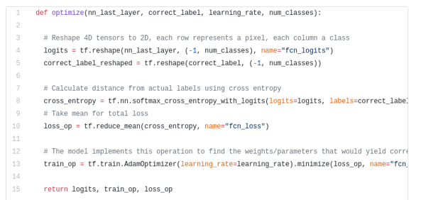
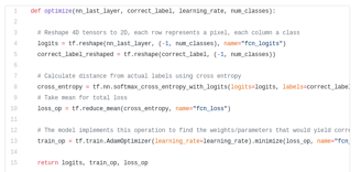
Optimize Function
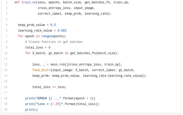
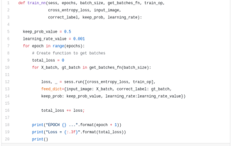
Step 4
Here we define the train_nn function, which takes in important parameters including number of epochs, batch size, loss function, optimizer operation, and placeholders for input images, label images, learning rate. For the training process, we also set keep_probability to 0.5 and learning_rate to 0.001. To keep track of the progress, we also print out the loss during training.
Step 5
Finally, it’s time to train our net! In this run function, we first build our net using the load_vgg, layers, and optimize function. Then we train the net using the train_nn function and save the inference data for records.
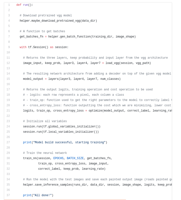
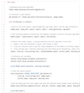
Run Function
About our parameters, we choose epochs = 40, batch_size = 16, num_classes = 2, and image_shape = (160, 576). After doing 2 trial passes with dropout = 0.5 and dropout = 0.75, we found that the 2nd trial yields better results with better average losses.

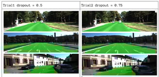
Training Sample Results
To see the full code, check out this link: https://gist.github.com/khanhnamle1994/e2ff59ddca93c0205ac4e566d40b5e88