Running-Algos
The 5 Fundamental Running Times in Computer Science
As a software engineer, there are many important things for you to take care of, like code readability, modularity, security, maintainability… Why worry about performance? Well, performance is like the currency through which we can do all the other things. For example, let’s say given 2 algorithms for a task, how can you find out which one is better? The naive way to do so is to implement both and run them for different inputs to see which one takes less time. However, there are problems with this approach:
For some inputs, one of the two algorithms performs better than the other.
For some inputs, one algorithm performs better on one machine and the other algorithm works better on other machines for some other inputs.
Asymptotic analysis is the idea that handles these issues in analyzing algorithms. In an asymptotic analysis, we evaluate the performance of an algorithm in terms of input size (we don’t measure the actual running time). We calculate, how does the time (or space) taken by an algorithm increases with the input size.
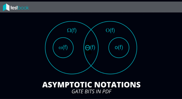
An algorithmic analysis is performed by finding and proving asymptotic bounds on the rate of growth in the number of operations used and the memory consumed. The operations and memory usage correspond to the analysis of the running time and space, respectively. Here are the 3 types of bounds most common in computer science:
Asymptotic Upper Bound (aka Big-Oh) — Definition: f(n) = O(g(n)) if there exists a constant c > 0 and a constant n_{0} such that for every n >= n_{0} we have f(n) <= c * g(n).
Asymptotic Lower Bound (aka Big-Omega) — Definition: f(n) = Omega(g(n)) if there exists a constant c > 0 and a constant n_{0} such that for every n >= n_{0} we have f(n) >= c * g(n).
Asymptotically Tight Bound (aka Big-Theta) — Definition: f(n) = Theta(g(n)) if there exists constants c_{1}, c_{2} > 0 and a constant n_{0} such that for every n >= n_{0} we have c_{1} g(n) <= f(n) <= c_{2} g(n).
Here the 2 major properties of these asymptotic growth rates:
Transitivity: if a function f is asymptotically upper-bounded by a function g, and if g in turn is asymptotically upper-bounded by a function h, then f is asymptotically upper-bounded by h. A similar property holds for lower bounds.
Sums of Functions: if we have an asymptotic upper bound that applies to each of 2 functions f and g, then it applies to their sum.
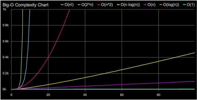
Out of these 3 bounds, computer scientists should focus mostly on Big-Oh Notation, which specifically describes the worst-case scenario, and can be used to describe the execution time required or the space used by an algorithm. It enables a software engineer to determine how efficient different approaches to solving a problem are. Let’s look at some common types of time complexities in Big-Oh Notation:
1 — O(1) Constant TimeConstant time algorithms will always take same amount of time to be executed. The execution time of these algorithm is independent of the size of the input. A good example of O(1) time is accessing a value with an array index.
void printFirstItem (const vector& array) {
cout << array[0] << endl;
}2 — O(n) Linear timeAn algorithm has a linear time complexity if the time to execute the algorithm is directly proportional to the input size n. Therefore the time it will take to run the algorithm will increase proportionately as the size of input n increases.
void printAllItems (const vector& array) {
for (int i = 0; i < array.size(); i++) {
cout << i << endl;
}
}3 — O(log n) Logarithmic TimeAn algorithm has logarithmic time complexity if the time it takes to run the algorithm is proportional to the logarithm of the input size n. An example is binary search, which is often used to search data sets:
int BinarySearch (const vector& array, int targetValue) {
length = array.size();
int minIndex = 0;
int maxIndex = length - 1;
int currentIndex;
int currentElement;
while (minIndex <= maxIndex) {
currentIndex = (minIndex + maxIndex) / 2;
currentElement = array[currentIndex];
if (currentElement < targetValue) {
minIndex = currentIndex + 1;
} else if (currentElement > targetValue) {
maxIndex = currentIndex - 1;
} else {
return currentIndex;
}
}
return -1; // If the index of the element is not found
}4 — O(n²) Quadratic TimeO(n²) represents an algorithm whose performance is directly proportional to the square of the size of the input data set. This is common with algorithms that involve nested iterations over the data set. Deeper nested iterations will result in O(n³), O(n⁴) etc.
for (int i = 0; i < 5; i++) {
for (int j = 0; j < 4; j++) {
// More loops
}
}5 — O(2^n) Exponential TimeO(2^n) denotes an algorithm whose growth doubles with each addition to the input data set. The growth curve of an O(2^n) function is exponential: starting off very shallow, then rising meteorically. An example of an O(2^n) function is the recursive calculation of Fibonacci numbers:
int Fibonacci(int number) {
if (number <= 1) return number;
return Fibonacci(number - 2) + Fibonacci (number - 1);
}